AP Biology · Unit 7 · Topic 7.2
Natural Selection
Two insects encounter the same environmental chemical. One breaks it down efficiently; the other accumulates enough to disrupt cell function. “One is better adapted” names an outcome but does not yet explain it. What differs inside their cells, how does that difference affect survival and reproduction, and what can their descendants inherit?
Connect the molecule to the organism
A phenotype is not limited to a visible feature. Enzyme activity, the abundance of a membrane transporter, and the timing of a response can also vary. A DNA difference might change a protein's amino acid sequence or alter how much protein a cell produces. Neither change is automatically useful: its consequences depend on what the molecule does and on the conditions the organism encounters.
For a hypothetical insect, imagine a regulatory allele that increases the amount of an enzyme that converts a particular environmental chemical to a less harmful product. With sufficient substrate, the extra enzyme could increase breakdown, reduce cellular damage, and improve survival to reproduction. Producing that protein also consumes resources. In an environment without the chemical, the protective benefit may disappear while a production cost remains.
This is a proposed causal mechanism, not evidence about an actual insect species. To test it, measure enzyme abundance, chemical breakdown, and reproductive contribution rather than inferring the entire chain from a DNA sequence alone. More protein is not always better: substrate availability and other limiting steps can prevent extra enzyme from improving performance.
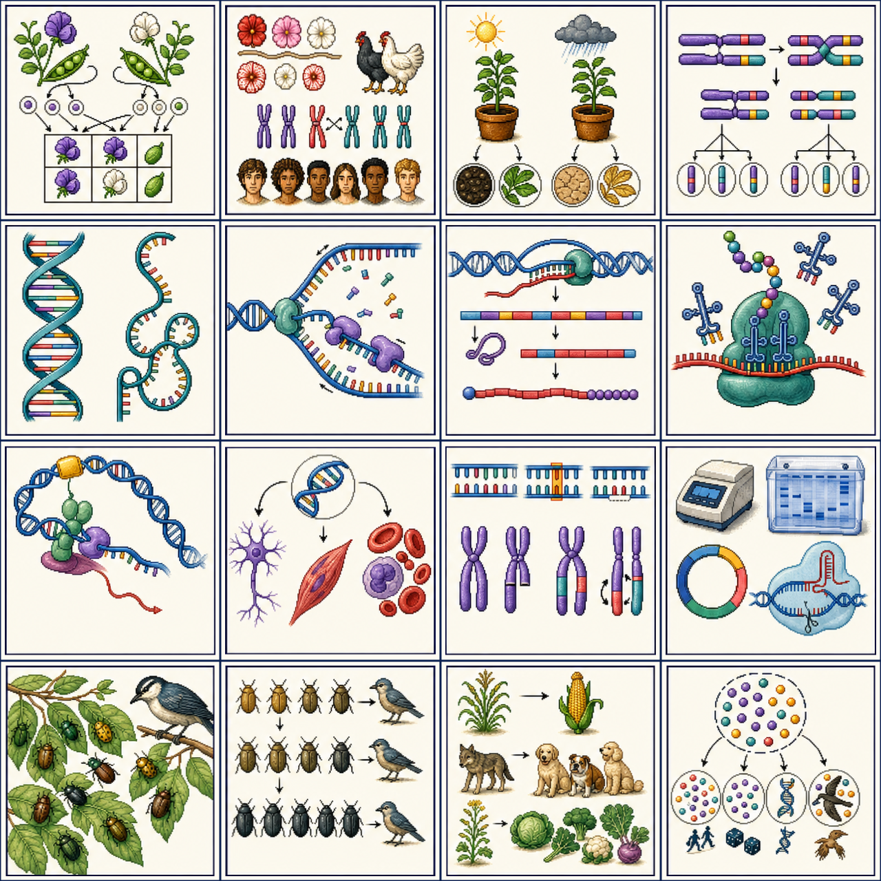
Separate inherited variation from a response to exposure
A genotype can produce different phenotypes in different environments. If exposure switches on enzyme production in every insect, that is an environmentally induced response; it does not establish that a new allele has appeared. Inherited differences in the ability to make that response can themselves be subject to selection.
Mutation supplies new alleles, while sexual reproduction reshuffles existing variation. Mutation is not directed toward a particular future benefit. Selection can increase a variant already present before an environmental change. An increase in resistance after exposure therefore does not, by itself, show that exposure created the resistance allele.
Selection can only distinguish variants through consequences that affect reproductive success in the relevant setting. A DNA difference with no such consequence may be neutral in that setting. Conversely, two different DNA changes can produce similar phenotypes; phenotype alone does not identify the responsible sequence.
A real connection: coat color and the surroundings
Research on rock pocket mice connects inherited coat-color variation to camouflage on different substrates. HHMI BioInteractive's account describes mostly light coats on light sand and mostly dark coats on dark rock, with predation providing a selective pressure. Genetic work also shows that similar dark phenotypes can arise through different genetic routes.
The explanatory chain is not “dark rock makes a mouse dark.” Inherited differences affect pigmentation; pigmentation affects conspicuousness against a background; predation can change opportunities to reproduce. A dark coat is not a context-free advantage. This research provides a biological example of the connection between molecular variation and selection, rather than a rule that one color or one allele must win everywhere.
External resource: HHMI BioInteractive — Natural Selection and Adaptation. The film and its classroom materials remain on the provider's site; they are not embedded or reproduced here.
Work from genotype counts, not a guessed equilibrium
Return to our invented insect model. At one autosomal locus, alleles R and r produce three genotypes. Assume RR has high enzyme abundance, Rr intermediate abundance, and rr low abundance. These relationships are stipulated for this example, not universal dominance rules. We follow the same closed cohort before and after exposure, with no reproduction, migration, or mutation during the interval.
| Genotype | Before exposure | Survival fraction | Surviving individuals | R copies among survivors |
|---|---|---|---|---|
| RR | 40 | 0.90 | 36 | 72 |
| Rr | 40 | 0.60 | 24 | 24 |
| rr | 20 | 0.20 | 4 | 0 |
Each diploid individual carries two copies of this locus. Before exposure, the 100 individuals contain 200 allele copies. RR individuals contribute two R copies each and Rr individuals one each. If \(p_R\) denotes the fraction of allele copies that are R:
After exposure, \(36+24+4=64\) individuals remain. Count their alleles again rather than keeping the original denominator:
R rises from 60% to 75% of allele copies among survivors. Yet the number of R copies falls from 120 to 96. An allele can become more frequent while becoming less numerous because the comparison is a share of a shrinking total.
Do not confuse the allele frequency with the fraction of individuals carrying R. Among survivors, carriers are RR or Rr: \((36+24)/64=0.9375\), or 93.75%. The R allele frequency is 75%, not 93.75%. Counting copies distinguishes these questions without requiring Hardy–Weinberg assumptions.
The result establishes a shift in the surviving cohort under the model. It does not by itself determine the next generation. If all survivors contribute equally to a large gamete pool and segregation is Mendelian, the expected R frequency in that pool is 0.75. Unequal mating success, fecundity, or later survival could change the final outcome; finite sampling also introduces variation.
Compare the same genotypes in two environments
Suppose a separate, otherwise comparable cohort is observed without the chemical. In this hypothetical comparison, RR, Rr, and rr have survival fractions 0.60, 0.80, and 1.00. A proposed explanation is a cost of enzyme production without a compensating protective benefit. The numbers alone do not prove that explanation.
Using the same starting counts without exposure gives 24 RR, 32 Rr, and 20 rr survivors. R's frequency is \([2(24)+32]/[2(76)]=80/152\approx0.526\), below its initial 0.60. The direction reverses between environments. Calling R simply a “good allele” discards the condition responsible for the difference.
To evaluate the proposed cost, compare otherwise similar genetic backgrounds and measure enzyme production and resource use. Other linked genetic differences could affect survival. A graph that fits a hypothesis is not the same as a test that rules out its alternatives.
Selection can change a distribution in different ways
For a quantitative phenotype, ask which values have greater reproductive success, not merely which values are common. A common phenotype can have low current fitness if conditions have recently changed.
| Pattern | Fitness comparison | Possible distributional response |
|---|---|---|
| Directional | One end is favored over the other. | The mean can shift toward the favored end. |
| Stabilizing | Intermediate values outperform both extremes. | The spread can narrow with little shift in the mean. |
| Disruptive | Both extremes outperform intermediate values. | The distribution can become more concentrated toward two ends. |
These are conditional predictions: the phenotype must have an inherited component for a sustained evolutionary response, and other processes can alter the result. Disruptive selection does not by itself demonstrate that two species have formed. Also distinguish a graph of fitness versus trait value from a graph of number of individuals versus trait value; their vertical axes answer different questions.
Use the evidence to make a bounded claim
A stronger explanation names an observed difference and follows its consequences. For the invented exposed cohort, “RR survived at 90%, compared with 20% for rr, shifting R from 0.60 to 0.75 among survivors” is supported. “R will reach 100% next generation” is not: we have not measured reproduction, and the other environment shows a possible disadvantage.
Replicated cohorts, comparable starting conditions, and an unexposed comparison help distinguish a repeatable genotype–environment relationship from chance. Following descendants tests whether the selected differences persist through inheritance. Neither a single association nor an appealing molecular story supplies all of that evidence.
Reason through the remaining gaps
1. Why is 60/64 not the R allele frequency among exposed survivors?
It counts individuals carrying at least one R. The denominator for an allele frequency is 128 copies of the locus, not 64 individuals. RR contributes 72 R copies and Rr contributes 24, giving \(96/128=0.75\).
2. The number of R copies declined. Does that contradict selection favoring R during exposure?
No. R declined from 120 to 96 copies, while r declined from 80 to 32. R was retained at a higher rate and its share increased. Absolute abundance and relative frequency are different measures.
3. What if the surviving rr insects each produce many more offspring than the RR insects?
The next generation need not preserve the survival-based ranking. Count each genotype's reproductive contribution and the alleles it transmits. The survival chart measures only one life-cycle component, not complete fitness.
4. Can an unchanged mean show that selection did not occur?
No. Stabilizing selection can reduce variation around approximately the same mean. Disruptive selection can also preserve a symmetric mean while changing the distribution's shape. Inspect the spread, frequencies across trait values, and reproductive data. Distribution shape alone does not prove the cause.
5. All exposed insects increase enzyme production. What additional evidence would connect that observation to evolution?
Establish inherited differences in production or responsiveness, test whether those differences predict reproductive contribution, and follow the inherited composition across generations. An induced response in existing individuals is not sufficient. A regulatory response can be useful without any allele-frequency change occurring during that observation.
Concept references: OpenStax Biology 2e: Population Genetics; OpenStax Biology 2e: Adaptive Evolution; HHMI BioInteractive: Natural Selection and Adaptation. Scope reference: College Board AP Biology Course and Exam Description, Topic 7.2. Explanations, insect scenarios, numerical data, diagrams, and questions were independently composed. These external references do not imply reuse permission; no source worksheets, illustrations, or videos are reproduced.
Official curriculum reference: College Board AP Biology course page. The explanation and worked example are independently written for this study site.