Prealgebra · Unit 9 · Topic 9.4
Experimental Probability and Fair Comparisons
Use observed event counts to calculate experimental probability, compare unequal trials with rates, pool compatible results, and interpret a percentage graph.
What an experiment can tell us
A spinner may have a blue region, but a drawing of the spinner does not tell us how often blue actually appeared in a set of spins. We can run trials and count. The result is an experimental probability, also called a relative frequency:
\[ \widehat{P}(\text{blue})= \frac{\text{number of spins that landed on blue}} {\text{total number of valid spins}}. \]
The hat reminds us that this is an estimate from observations, not a guarantee for the next spin. The denominator must be greater than zero. Since the blue count cannot exceed the total count, an experimental probability is between 0 and 1. Multiply by 100 to express it as a percentage. The fraction and percentage have no physical unit.
A theoretical probability starts with a model instead. If blue covers exactly one of four equal sectors and the spinner is equally likely to stop in each sector, the model gives \(P(\text{blue})=1/4=25\%\). An experiment with 20 spins need not produce exactly five blue results. Conversely, seeing five blue results in 20 spins does not prove that the spinner has four equal sectors. The model and the observations answer related, but different, questions.
Compare two runs with different totals
Suppose one run records 17 blue results in 50 spins and another records 9 in 20. We will call these Run A and Run B. “Blue” and “one valid spin” must mean the same thing in both runs.
| Run | Blue spins | Other spins | Total spins | Experimental probability of blue |
|---|---|---|---|---|
| A | 17 | 33 | 50 | \(17/50=0.34=34\%\) |
| B | 9 | 11 | 20 | \(9/20=0.45=45\%\) |
Run A has more blue results (17 versus 9), but it also has many more chances to produce one. Dividing each count by its own total gives a fairer comparison: blue appeared in 34 of every 100 spins at A's observed rate, compared with 45 of every 100 at B's observed rate. These “per 100” statements rescale the rates; they do not claim that either run actually contained 100 spins.
\[ \widehat{P}_A=\frac{17}{50}=0.34,\qquad \widehat{P}_B=\frac{9}{20}=0.45. \]
\[ 0.45-0.34=0.11=11\text{ percentage points}. \]
The difference is 11 percentage points, not simply “11 percent more.” A percent increase would use A's rate as its denominator and answer a different question.
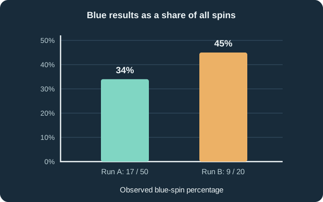
Before trusting this comparison, check the conditions. Were both runs made with the same spinner? Was “blue” defined the same way? Were all spins counted, including inconvenient results? If the conditions differ, a difference in rates may be due to the procedure rather than the spinner. Even under identical conditions, random variation can produce different rates.
Combining runs is not the same as averaging their percentages
If A and B are separate, nonoverlapping runs under comparable conditions, they can be pooled. Add the blue counts, then add the trial counts:
\[ \widehat{P}_{\text{combined}} =\frac{17+9}{50+20} =\frac{26}{70} =\frac{13}{35} \approx 0.3714 \approx 37.1\%. \]
Why not calculate \((34\%+45\%)/2=39.5\%\)? That would give the 20-spin run and the 50-spin run equal influence, as though they contained the same number of observations. The combined rate is a weighted average:
\[ \frac{50(0.34)+20(0.45)}{50+20} =\frac{17+9}{70} =\frac{26}{70}. \]
Its value lies between 34% and 45%, closer to A's rate because A contributed more trials. Pooling is inappropriate if the runs use different events or incompatible procedures; the arithmetic would hide an important distinction.
What a difference does—and does not—show
The observed rates tell us exactly what happened in these runs: A had 34% blue and B had 45% blue. They do not, by themselves, prove that one spinner is biased or that the true chance changed. A smaller run can fluctuate noticeably from one repetition to the next. More trials under consistent conditions generally give a steadier estimate, but no particular sample size forces the observed rate to equal the theoretical chance exactly.
If the claim is that a spinner is “fair,” first define what fair means. For a spinner with equal-sized color sectors, compare the results with the model based on those sectors. Without knowing the blue area's size or the intended design, 34% and 45% alone cannot establish unfairness.
To check your understanding, imagine a third run with 12 blue results in 40 spins. Its experimental probability is \(12/40=30\%\). It has more blue results than B (12 versus 9), yet a lower blue rate (30% versus 45%). This is the same reason we compare rates, not raw counts, whenever totals differ.
Further reading
The distinction between theoretical and empirical probability, and the importance of comparable trial conditions, were checked against OpenStax Contemporary Mathematics §7.5. Relative frequency as a count divided by a total was checked against OpenStax Introductory Statistics 2e §1.3. The explanation, examples, table, and graph here were independently written or drawn; textbook prose, exercises, and artwork were not reproduced.