Prealgebra · Unit 9 · Topic 9.1
Reading Tables and Data Graphs
Read tables, time-series line graphs, and category bar charts; calculate totals and changes while checking axes, units, and misleading scales.
A table answers a different question from a graph
Suppose a small study room records daily visits for one week. The figures below are invented for this lesson, not measurements from this website. A table gives each exact count; a graph helps you notice where the count rose or fell. Before either one can answer a question, check what a row or point represents. “Visits on Tuesday” is not the same as “visits so far by Tuesday.”
| Day | Daily visits (people) |
|---|---|
| Monday | 12 |
| Tuesday | 18 |
| Wednesday | 15 |
| Thursday | 21 |
| Friday | 19 |
Each row pairs a day with its count. The unit people belongs to the counts, not the day names. Tuesday has 18 visits; it does not mean 18 more than Monday. To find the change from Monday to Tuesday, subtract the earlier count from the later one:
\[ \text{change}=18-12=+6\text{ people}. \]
From Tuesday to Wednesday, the same rule gives \(15-18=-3\) people. The negative sign says the daily count fell; it does not mean a negative number of people visited. Across all five days, the total is
\[ 12+18+15+21+19=85\text{ visits}. \]
The net change in daily count from Monday to Friday is different: \(19-12=+7\) people. Adding all the adjacent changes gives \(+6-3+6-2=+7\), the same result. Do not use \(85\) when the question asks only how much the daily count changed between the first and last day.
Read a line graph as ordered pairs
The graph below plots the same table. The horizontal axis lists days in time order; the vertical axis measures daily visitors in people and starts at 0. Each dot is one recorded count: Monday is \((\text{Mon},12)\), Tuesday is \((\text{Tue},18)\), and so on. One vertical grid interval represents 5 people, so Tuesday's dot lies between 15 and 20 rather than exactly on a gridline.
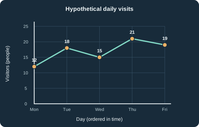
The highest observed daily count is 21 on Thursday and the lowest is 12 on Monday. The difference is \(21-12=9\) people. The line rises from Monday to Tuesday, falls on Wednesday, rises to Thursday, and falls again on Friday. It would be inaccurate to say “visits rose every day” merely because Friday's count exceeds Monday's.
The connecting segments are a visual guide between discrete daily observations. They do not prove what happened at noon between observations, and the up-and-down pattern does not explain why the numbers changed. A cause would require additional evidence.
Sometimes a question asks for a percent change instead of a difference in people. For Monday to Tuesday, use the starting value as the denominator:
\[ \text{percent change}=\frac{18-12}{12}\times100\%=50\%. \]
The absolute change is 6 people; the relative change is 50%. Stating “a 50% increase” without saying from which starting day leaves out essential information.
Categories call for bars, not a time path
Now consider a separate, also invented, survey of 45 students choosing one after-school activity: 12 chose Math, 18 Science, and 15 Art. The categories are not successive moments, so a line connecting them would suggest a time sequence that does not exist. A bar chart gives each category its own bar; the height encodes the number of students. The bars are separated because the category names are distinct groups.
| Activity chosen | Students (people) |
|---|---|
| Math | 12 |
| Science | 18 |
| Art | 15 |
| Total | 45 |
Science exceeds Math by \(18-12=6\) students. The ratio of their counts is \(18/12=1.5\), so Science has one and a half times as many students as Math. This numerical comparison is more reliable than judging which colored rectangle looks tallest.
When an axis exaggerates a difference
Both bar charts below use that same survey. The left-hand chart starts the vertical axis at 0; the right-hand chart starts at 10. On the right, the visible portion of Science's bar spans \(18-10=8\) units, while Math's spans \(12-10=2\) units. Those visible pieces have a 4-to-1 height ratio even though the actual counts have only an \(18/12=1.5\)-to-1 ratio.
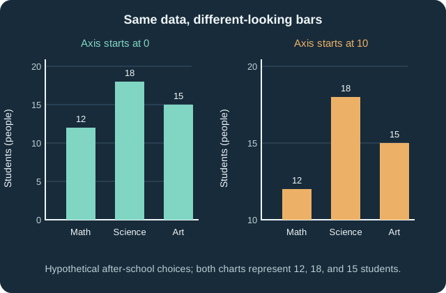
Starting an axis above zero is not automatically forbidden, but bar lengths are easiest to compare fairly from a zero baseline. If a chart uses a cut-off axis, it should make that choice unmistakable, and the reader should compare the printed values rather than the visible bar lengths. Also check whether tick intervals are equal and whether a label means a raw count, a percentage, or something else; \(18\) people and \(18\%\) are not interchangeable.
A blank table cell is not necessarily zero. If Wednesday's count were missing, we could not conclude it was 0 or draw a trustworthy point there without more information. Similarly, a graph can show an association or trend without revealing a cause. Begin with the title, population and time period, axis labels, units, and scale; then use the actual numbers to answer the question asked.
Further reading
The treatment of frequencies, bar charts, and ordered data was checked against OpenStax Introductory Statistics 2e §1.3, §2.1, and OpenStax Contemporary Mathematics §8.2. The prose, hypothetical datasets, worked calculations, tables, and SVG graphs here were independently created; textbook text, exercises, and artwork were not reproduced.