Prealgebra · Unit 9 · Topic 9.3

Sample Spaces and Simple Probability

Build sample spaces, count equally likely outcomes, use complements, and read a probability bar graph without confusing outcomes with event categories.

Decide what counts as one outcome

If we choose one card from ten numbered cards, an outcome can be the number on the chosen card. If we toss a coin twice, an outcome must record both tosses in order. Before counting probabilities, state exactly what the experiment produces; otherwise a list may quietly omit a possibility or treat unequal possibilities as equal.

The sample space \(S\) is the set of all possible outcomes of the experiment. An event \(E\) is a collection of outcomes in \(S\) that satisfy a condition. For a finite sample space whose individual outcomes are equally likely, we can count:

\[ P(E)=\frac{\text{number of outcomes in }E}{\text{number of outcomes in }S} =\frac{n(E)}{n(S)},\qquad n(S)>0. \]

Here \(n(E)\) means the number of distinct outcomes in the event. Probability has no unit. Because the event can contain anywhere from none to all of the sample space, \(0\leq P(E)\leq1\). An impossible event has probability 0; a certain event has probability 1.

One draw from ten numbered cards

Suppose ten identical cards are numbered 1 through 10 and shuffled so each is equally likely to be drawn. The sample space is

\[ S=\{1,2,3,4,5,6,7,8,9,10\}. \]

Let \(E\) mean “draw a number greater than 6.” The favorable outcomes are \(E=\{7,8,9,10\}\), so

\[ P(E)=\frac{4}{10}=\frac{2}{5}=0.4=40\%. \]

The word greater matters: 6 is not included. The complement \(E^{c}\) contains everything in \(S\) that is not in \(E\), namely \(\{1,2,3,4,5,6\}\). Thus

\[ P(E^{c})=\frac{6}{10}=\frac35,\qquad P(E)+P(E^{c})=\frac25+\frac35=1. \]

Every draw either is greater than 6 or is not; there is no third case and no overlap. This is why \(P(E^{c})=1-P(E)\). For example, “at most 6” is the complement of “greater than 6,” not “less than 6.”

Two tosses: four ordered outcomes, not three

Now toss a fair coin twice, assuming the tosses do not affect one another. Use \(H\) for heads and \(T\) for tails. Recording the first toss followed by the second gives

\[ S=\{HH,HT,TH,TT\}. \]

The grid below lists the first toss by row and the second by column. Each cell has probability \(1/4\): one specified result on the first fair toss has probability \(1/2\), and the independent specified result on the second has probability \(1/2\), so \((1/2)(1/2)=1/4\).

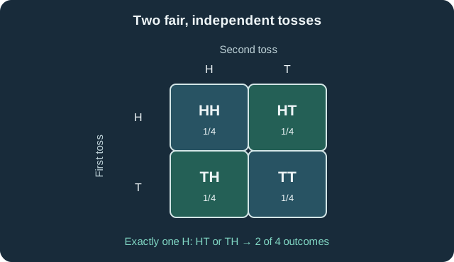
Two-by-two sample-space grid for two fair independent coin tosses. Rows are first toss H or T; columns are second toss H or T. The four equally likely cells HH, HT, TH, TT each have probability one fourth. HT and TH are highlighted. — Original sample-space diagram. The order distinguishes \(HT\) from \(TH\), even though each has one head.

Let \(F\) mean “exactly one head.” Both \(HT\) and \(TH\) satisfy that condition, so

\[ F=\{HT,TH\},\qquad P(F)=\frac24=\frac12. \]

Counting “one head” as only one outcome would confuse the description of an event with the elementary outcomes that make it happen.

For “at least one head,” we could list \(HH,HT,TH\) and obtain \(3/4\). Or count the easier complement, “no heads,” which is only \(TT\):

\[ P(\text{at least one head})=1-P(TT)=1-\frac14=\frac34. \]

Both routes agree. This is a useful check whenever a complement is simpler to count than the requested event.

Why the probability graph is not flat

Group the four equally likely outcomes by the number of heads. There is one outcome with zero heads (\(TT\)), two with one head (\(HT,TH\)), and one with two heads (\(HH\)). Therefore

\[ P(0\text{ heads})=\frac14,\quad P(1\text{ head})=\frac24=\frac12,\quad P(2\text{ heads})=\frac14. \]

The three bars below represent these theoretical probabilities. The horizontal axis names the number of heads; the vertical axis is probability from 0 to \(1/2\), marked in steps of \(1/4\). Their heights add to \(1/4+1/2+1/4=1\), accounting for every outcome.

Theoretical probability bar graph for zero, one, or two heads in two fair independent coin tosses. Bars have heights one fourth, one half, and one fourth on a probability axis from zero to one half. — Original theoretical graph, not results from an actual experiment. The middle category is twice as likely because it contains two equally likely ordered outcomes.

The categories 0, 1, and 2 heads are not equally likely, even though \(HH,HT,TH,TT\) are. Dividing “one favorable category” by “three categories” would give \(1/3\), an incorrect answer. Count equally likely elementary outcomes first, then combine them into the event the question asks about.

When simple counting does not apply

The fraction \(n(E)/n(S)\) works only when the outcomes being counted have equal chances. Imagine a spinner with one red sector covering one quarter of the circle and a blue sector covering the other three quarters. The sample space of colors is \(\{\text{red},\text{blue}\}\), but the colors are not equally likely: \(P(\text{red})=1/4\), not \(1/2\). For unequal outcomes, use their actual probabilities rather than counting labels as if they had equal weight.

Likewise, a prediction of \(P(F)=1/2\) does not promise exactly one head in half of any four observed trials. It describes the chance under the stated fair-and-independent model. Observed frequencies from repeated trials can vary; they are a separate kind of evidence.

When solving a new problem, list the possible outcomes in a way that matches the experiment, identify the event as a subset, and check whether equal likelihood is justified. A probability below 0 or above 1 signals an error, and the complement provides a second check when it is easy to count.